
Outline of Activities Performed During Stage 1
For 2018, three tasks part of WP 1 were performed. As a result, a complete time and frequency domain description was obtained for the electron density and ionospheric tilts at Wallops Island in June and November 2015. Figures 1 and 2 show the full extent of the data, interpolated to a fixed height grid.
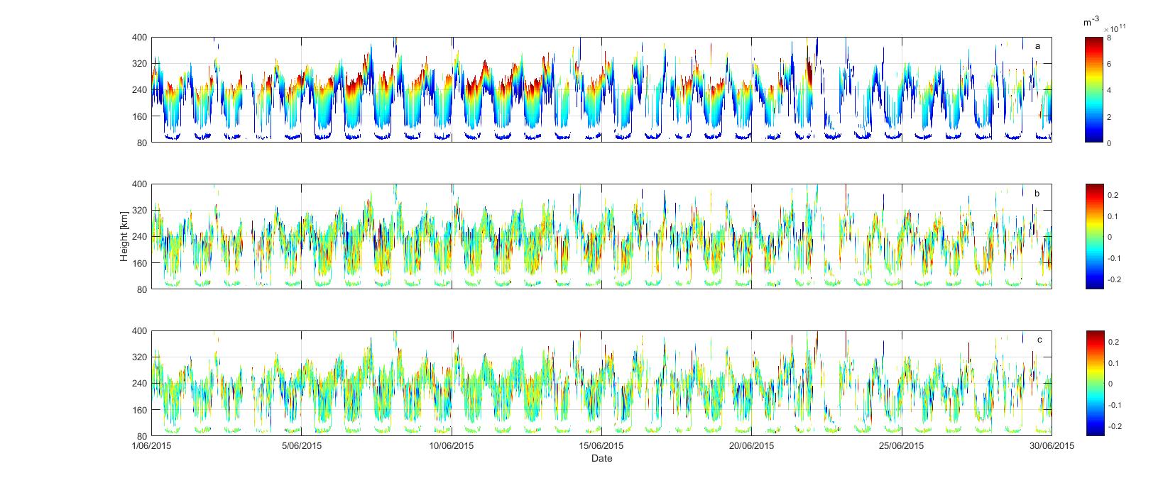
Figure 1. Dynasonde data from Wallops Island for June 2015: a. Electron density, b. Zonal tilt and c. Meridional tilt.
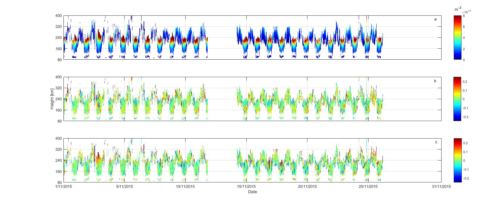
Figure 2. Same as fig. 1, but for November 2015.
In addition to the raw measurements, a detrended version of the electron density was obtained. The detrending procecdure is designed to separate the effects due to solar and geomagnetic forcings (the background component) from TIDs (the perturbation component). Figure 3 demonstrates this on a 24-hour data subset.

Figure 3. Example of a detrending result, for a 24-hour dataset on 5-6 June 2015, at 200 km altitude.
To better highlight the impact of AGWs, two 24-hour datasets are displayed in figures 4-5.
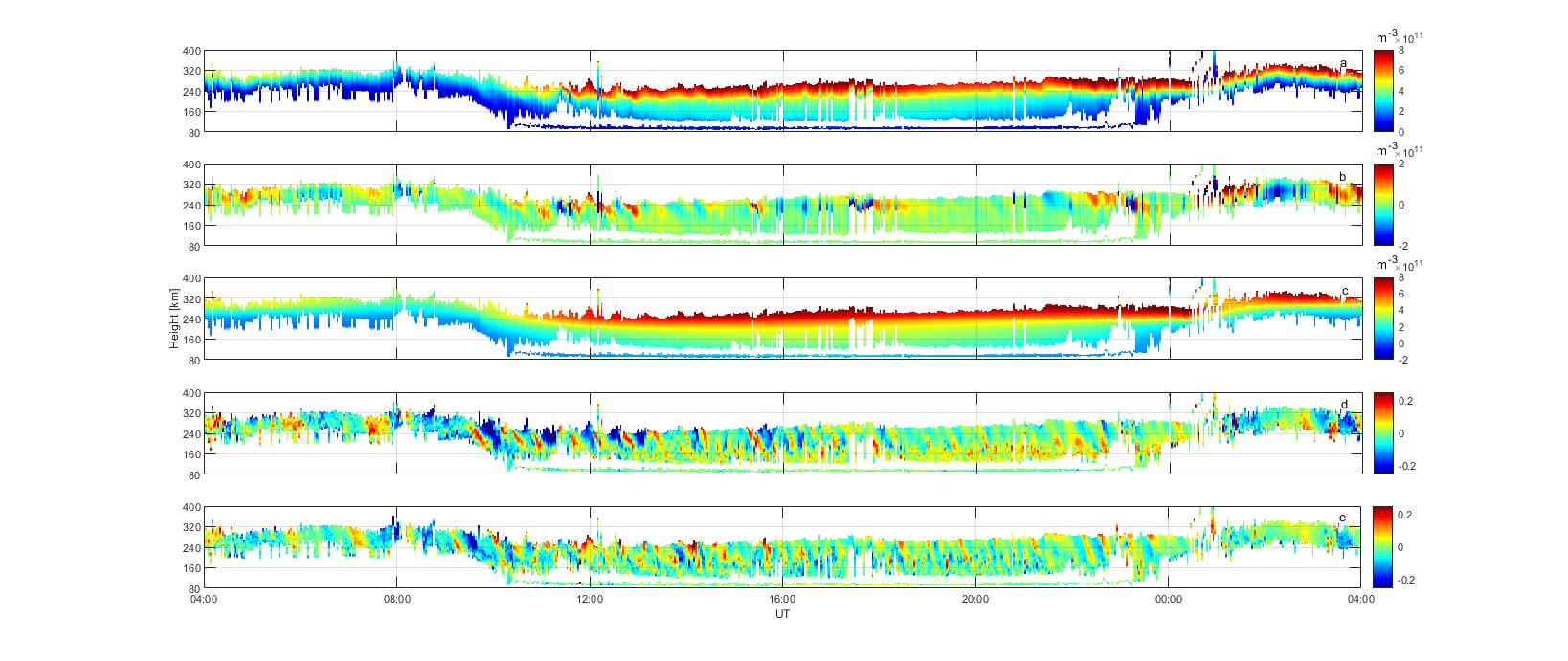
Figure 4. Time domain description of the ionospheric parameters on June 6th, 2015: a. Electron density, b. electron density perturbations, c. electron density background, d. zonal tilt and e. meridional tilt.
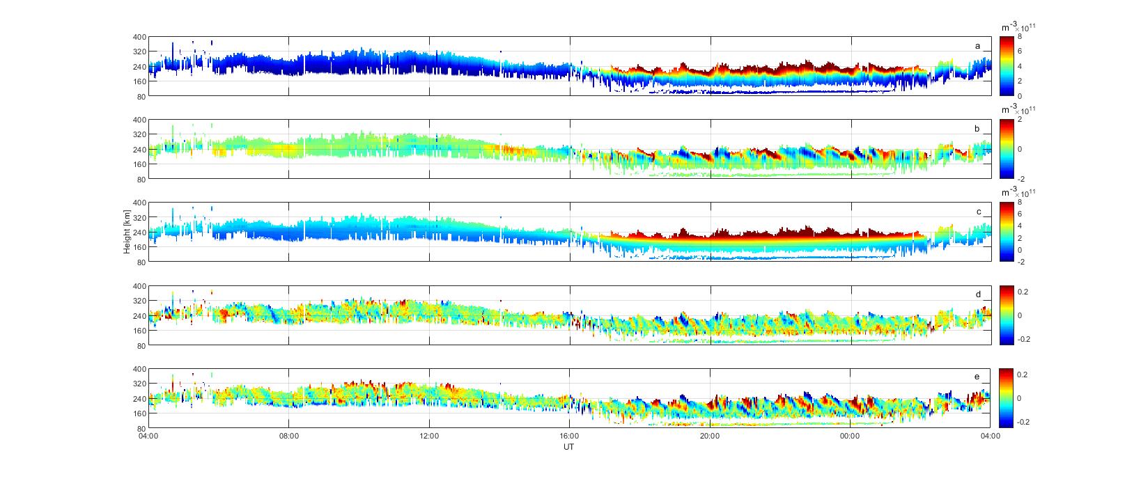
Figura 5. Same as fig. 4, but for November 17th, 2015.
Using the spectral analysis technique described by Negrea and Zabotin (2016), the detrended electron density and ionospheric tilts are analyzed. An example of power spectra is shown in figure 6. A 2-hour sliding window is used, with a 10-min step to capture the temporal evolution of the power spectrum.
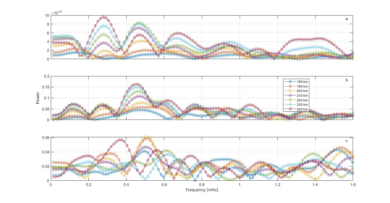
Figure 6. Example of a spectral analysis result for a 2-hour interval on June 6th, 2015, at the altitudes listed in the legend. The data used was: a. Electron density perturbations, b. zonal tilt and c. meridional tilt.
Figures 7-9 show the time and altitude variation of the power determined at three different frequencies.

Figure 7. Time and altitude variation (for June 2015) of spectral power at 0.26 mHz (equivalent to 63 min period) for a. Electron density perturbation, b. zonal tilt and c. meridional tilt.
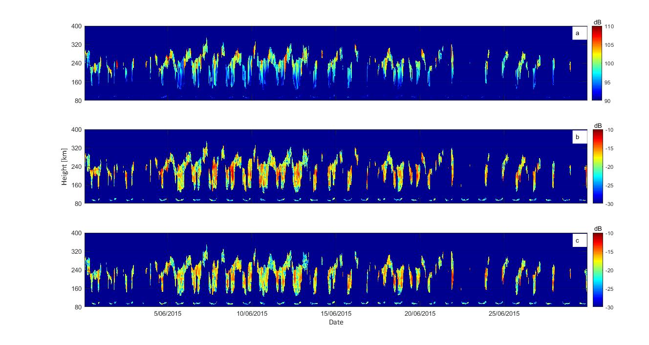
Figure 8. Same as fig. 7, but for a frequency of 1.09 mHz (equivalent to a 15 min period).

Figure 9. Same as fig. 7, but for a frequency of 1.65 mHz (equivalent to a 10 min period).